Download raw sensor data

The ACM DEBS 2013 Grand Challenge is the third in a series of challenges that seek to provide common ground and evaluation criteria for a competition aimed at both research and industrial event-based systems. The goal of the Grand Challenge competition is to implement a solution to a problem provided by the Grand Challenge organizers.

The DEBS Grand Challenge series provides problems that are relevant to the industry at large, as they allow for evaluation of event-based systems using real-life data and queries.

Participants in the DEBS 2013 Grand Challenge have to submit (1) a six-page paper in ACM SIG proceedings format that outlines the solution, highlighting its innovative aspects and presenting the evaluation method; and (2) a demonstration of the system – in the form of either a video or a screencast. All submissions are subject to a peer review process. Authors of all accepted submissions will be invited to present their systems during the DEBS 2013 Conference. Upon the explicit consent from the Challenge participants, authors’ solutions will be included in the global ranking.

The winner of the Grand Challenge will be announced and awarded during the conference banquet. The global ranking is based on the peer review scores and how the solution performs. Assessment of that performance is based on the throughput and latency of the system under the assumption of result correctness.

Problem description

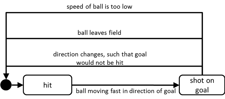
With the Grand Challenge, we seek to demonstrate the suitability of event-based systems for providing real-time complex analytics on high-velocity sensor data. One typical use case is the analysis of a soccer match. The data for the DEBS 2013 Grand Challenge originates from a set of wireless sensors embedded in the players’ shoes and the ball, which recorded the entire soccer game. The real-time analytics include the continuous computation of statistics relevant for spectators (ball possession, shots on goal) as well as coaches and team managers (running performance analysis of team members).

Data 

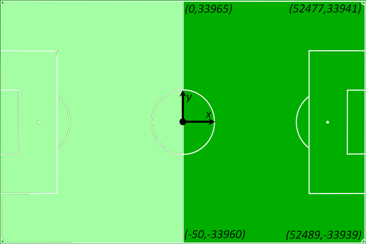
The data used in this year’s DEBS Grand Challenge was collected by a real-time locating system deployed on the field at the soccer stadium in Nuremberg, Germany. Data originated from sensors located near the players’ shoes (1 sensor per leg) and in the ball (1 sensor). The goalkeeper was equipped with two additional sensors, one on each hand. The sensors near the players’ shoes and on the goalkeeper’s hands produced data at a frequency of 200 Hz, while the sensor in the ball produced data at 2000 Hz. The total data flow reached roughly 15,000 position events per second, with each of these events describing the position of a given sensor in a three-dimensional coordinate system. The center of the playing field is at the coordinates (0, 0, 0) – see Figure 1 for the field’s dimensions and the coordinates for the kickoff. The event schema is as follows:

sid, ts, x, y, z, |v|, |a|, vx, vy, vz, ax, ay, az

where sid is the ID of the sensor that produced the position event, ts is a timestamp in picoseconds, e.g. 10753295594424116 (whereby 10753295594424116 designates the start of play and 14879639146403495 the end of the game), x, y, z describe the position of the sensor in mm (the origin is the middle of a full-size soccer field), and |v| (in μm/s), vx, vy, vz describe the direction of a vector with a size of 10,000. Hence, the speed of the object in x-direction in SI units (m/s) is calculated using the formula:

v’x = |v| * vx * 1e-4 * 1e-6

(vx in m/s is derived by |v| * 1e-10 * vx) and |a| (in μm/s²), ax, ay, az describe the absolute acceleration and its constituents in three dimensions (the acceleration in m/s² is calculated in a way similar to velocity). The acceleration does not include gravity, i.e. |a| is zero when the ball is at a fixed position and not 9.81 m/s².

In addition to the sensor data, we also provide a separate data stream for referee events, which include when the game is paused and resumed as well as the time and player IDs (player_ids) for substitutions.

Mapping of the relationships between player_id and team_id as well as between sensor_id and player_id is provided in the metadata file.
The game in which the data was collected was played on a half-size field with teams of seven players each. Each half of the game lasted thirty minutes. We assumed that the data would arrive at the test system with no delays or omissions.

Raw sensor data for the game can be downloaded from:
http://www2.iis.fraunhofer.de/sports-analytics/full-game.gz (2.6 GB)

All data has been aggregated into a single file and sorted by time stamp. The video recording of the game (vertical view, static camera) can be downloaded from:

http://www2.iis.fraunhofer.de/sports-analytics/RedFIR_2012_1.mov (1st half, 1.7 GB)

http://www2.iis.fraunhofer.de/sports-analytics/RedFIR_2012_2.mov (2nd half, 1.7 GB)

The metadata file containing the players’ names and associated transmitter IDs, detailed field coordinates, etc., can be downloaded here (10 kB).

Game stoppages and statistics regarding ball possession and shots on goal can be downloaded from: http://www2.iis.fraunhofer.de/sports-analytics/referee-events.tar.gz (10 kB)

These statistics were compiled manually and can serve as an aid in validating the respective query results.

Query 1: Running performance

This query aims to calculate the running performance of each player currently participating in the game. The following levels of intensity are defined in the system: standing (0–1 km/h), trot (up to 11 km/h), low-speed run (up to 14 km/h), medium-speed run (up to 17 km/h), high-speed run (up to 24 km/h), and sprint (faster than 24 km/h). Figure 2 shows the possible transitions between different levels, which need to be recorded for the running performance analysis.

The running performance query should return two categories of results: (1) current running statistics and (2) a set of aggregate running statistics. The current running statistics should be returned at a defined point in time with a maximum frequency of 50 Hz and must contain the following information:

ts_start, ts_stop, player_id, intensity, distance, speed

where ts_start represents the start of the measurement, ts_stop the end of the measurement, player_id the identity of the player, intensity the intensity level of the run, distance the length of the run (in the horizontal plane only) between ts_start and ts_stop, and speed the average speed over the measured distance of the run at a given intensity.

The aggregate running statistics must contain the following information:

ts, player_id, standing_time, standing_distance, trot_time, trot_distance, low_time, low_distance, medium_time, medium_distance, high_time, high_distance, sprint_time, sprint_distance

where ts represents the time stamp of the latest statistics update, player_id serves as the player identifier, xxx_time is the time the player spent at xxx intensity (in milliseconds), and xxx_distance is the distance covered at xxx intensity. The aggregate running statistics must be calculated for four different time windows: 1 minute, 5 minutes, 20 minutes and the whole game duration. For each window, events must be transmitted at a frequency of 50 Hz. As a result, the system will return four aggregate running statistics streams, one for each window. Moreover, every run that maintains a particular intensity for less than 1 second must be counted as part of the subsequent run that maintains its intensity for more than 1 second. For example, if a player is at the trot level for a longer period, then at the low-speed run level for 0.8 seconds, and then at a medium-speed run for a longer period, the duration of the low-speed run is to be added to the duration of the medium-speed run.

Please note that the requirement to count only intensity levels active for at least 1 second requires you to delay the output until a reliable measurement has been made

Query 2: Ball possession

The goal of this query is to calculate the ball possession for each of the players as well as for the team as a whole. A player (and thereby their team) is said to have possession whenever the ball is in close proximity (less than 1 meter distance between the ball sensor and the player’s closest sensor) and the player kicks it (the ball’s acceleration peaks). The ball stays in their possession until another player kicks it, the ball leaves the field, or the game is stopped. Ball possession is calculated as the time between initial contact with the ball (kick) and the last contact with the ball (kick). The ball may leave the player’s proximity but still stay in their possession.

The ball counts as “kicked” if its (transmitter’s) distance from a player’s foot (transmitter) is less than 1 meter and its acceleration reaches a value of at least 55 m/s². This value depends heavily on the fitness of the players – professional players are more likely to achieve values of up to 100 m/s². It may be appropriate to apply a mean filter to the acceleration values in order to get better detection performance.

The ball possession query should return two classes of results in the form of data streams: (1) ball possession per player and (2) ball possession per team. The ball possession per player stream should contain the following information:

ts, player_id, time, hits

where the ts is the latest time stamp of the event which led to an update of ball possession, player_id is the player identifier, time is the total time of ball possession for a given player, and hits is the total number of ball contacts of a given player.
The ball possession per team stream must contain the following statistics:

ts, team_id, time, time_percent

where ts is the time stamp of the last event to cause an update to the team’s ball possession, team_id is the team identifier, time is the total duration of ball possession for a given team, and time_percent is a given team’s ball possession as a percentage of the total ball possession time for both teams. Ball possession per team must be calculated for four different time windows: 1 minute, 5 minutes, 20 minutes and the whole game duration. As a result, the system will return four aggregate streams of ball possession statistics, one for each window.

The system may generate statistics streams at a maximum frequency of 50 Hz.

Query 3: Heat map

The goal of this query is to calculate statistics for how long each of the players spent in which region of the field. For this purpose, we define a grid with X rows parallel to the x-axis and equal-size Y columns along the y-axis. The parameters X and Y should be implemented with the following values: 8 and 13 (a grid of 104 cells), 16 and 25, 32 and 50, 64 and 100 (a grid of 6,400 cells), respectively. The system should return results for all parameter settings in parallel but separate data streams.

For each cell and each player, the system must provide the percentage of time that the player spent in that specific cell over four different time windows: 1 minute, 5 minutes, 10 minutes and the whole game duration. As a result, the system will return 16 data streams for each of the windows and all the grid parameters.
Each stream must be updated once per second and contain the following information:

ts, player_id, cell_x1, cell_y1, cell_x2, cell_y2, percent_time_in_time_cell

where ts represents the time stamp of the latest statistics update, cell_x1, cell_y1, cell_x2, cell_y2 are the coordinates of the lower left and upper right corners of the cell, player_id is the player identifier, and percent_time_in_time_cell is the percentage of time that the player spent in the cell during the period specific to the data stream (0.00%–100.00%).

Query 4: Shots on goal

The aim of this query is to detect when a player shoots the ball in an attempt to score a goal. A shot on goal is defined as any shot that would hit (or barely miss) the goal of the opposing team. Note that this includes unsuccessful attempts that are blocked by a player or saved by the goalkeeper, for example.

Below we provide suggestions for the implementation of shot detection. However, we also allow alternative implementations that yield good results (i.e. closely resemble the result lists provided in referee-events.tar.gz).

Figure 5 gives an overview of suggested states and transitions of shot detection. A shot is detected if the player <player_id> kicks the ball with a minimum acceleration of 55 m/s², and the ball’s projected trajectory would move it into the opponents’ goal area within 1.5 seconds after contact. The goal areas are defined as rectangles with the following coordinates:

Goal area, team 1: x > 22578.5 and x < 29898.5, y = 33941.0, z < 2440.0 
Goal area, team 2: x > 22560.0 and x < 29880.0, y = -33968.0, z < 2440.0

Please note that the player’s kick distorts the speed values of the ball. To compensate for this, a Kalman filter is used to preprocess the data, which then stabilizes over time. The computation of the ball’s trajectory may take this into account. To allow for corrective measures, we require only that the shot be detected at the latest when the ball has moved 1 meter away from the location where contact was made.

The Challenge allows participants to decide the degree to which they incorporate the physics of a flying ball into their trajectory calculations. A baseline solution that simply extrapolates the motion vector is acceptable. However, more accurate computations of the ball movement (e.g. those that take gravity into account) would be greatly appreciated.

For the duration of the shot (i.e. as long as the “shot on goal” state in Figure 5 is active), the data stream should be updated with motion values of the ball and the ID of the shooting player:

ts, player_id, x, y, z, |v|, vx, vy, vz, |a|, ax, ay, az

The data stream should be updated at the frequency of the sensor data until an exit condition is met. Exit conditions are (a) the ball leaves the field or (b) the direction changes such that it would no longer enter the goal area.

1.     Will there be a single file for all sensors or a separate file for each sensor (I assume the latter)? A separate file for each, but I will provide a replay unit that opens the data files and replays the position streams in real time. For that we need to define the data format. Should the data be sent via a connector or something like that?

2.     What units are position, speed and acceleration in? Is that clear now? I can further clarify why the units seem to be so strange for the actual problem description.

3.     How can we identify which sensor belongs to which player (shoe) and which one is the ball sensor (based on the file name, I presume)? I will provide an XML for that, ok? Or can we just specify that in text? Maybe that would be easiest…

4.     Can we assume that the data will arrive at the test system in order and without any omissions? Yes.

5.     Figure 1 – what is the definition of the active/inactive state of a player? How can such a state be detected using the sensor data? I think we can omit that. “Active player” is a player that participates in the game, i.e., a player that is not a substitute. Of course, there might be substitutions during the game. We’re getting many players from the club.

6.     Description of Query 1: Fraunhofer’s analysis of running performance includes players in the tracking state. How can such a state be detected using the sensor data? I think we can omit that. Sometimes the tracking function doesn’t work and positions are missing. And when tracking resumes, then the velocities are corrupt, and that would ruin the running performance analysis. I hope that that’s not the case for us.

7.     Query 1 – Running performance: What is the purpose of the min./max./avg. distance for the intensity parameter? This is statistical information about the distances for which certain players remain at certain levels of intensity. For example, while most sprints are very short, low-speed runs are considerably longer.

8.     Query 1 – Running performance: What is the purpose of the min./max./avg. speed for the intensity parameter? This is actually a mistake, and they shouldn’t be part of the running performance analysis. These values are of interest as regards the individual players and the teams relative to the time windows.

9.     Query 2 – Ball possession. How can we identify which players belong to which team? Configuration file as above?

10.  Query 2 – Ball possession. What exactly does “ball proximity” mean? That the distance between the player and the ball is no more than 1 meter.

11.  Query 2 – Ball possession. How can we detect that a player has kicked the ball? When the ball sensor transmits an acceleration peak.

12.  How do we detect a pause in the game (foul, offsides, etc.)? We could manually embed referee events in the data flow for that. Would that be ok? Maybe just an event like “whistle-blow”…

13.  Query 2 – Ball possession. Why is information on ball proximity necessary? We use this as a sub-query to detect the players that are near the ball. But we don’t need to evaluate that at the time of the ball’s acceleration peak. I think we should remove that “restriction.” That’s how we do it, but it’s perhaps not very efficient. Maybe we can find a better way.

The test match is currently scheduled to start at 5 p.m. on November 7, 2012.